New Path Tracer

In September I decided to challenge myself to write a path tracer in C++ without referring to any books, articles or tutorials, and rely on just what I have learned or can derive by myself. After a few months I’ve implemented a bunch of features and am pretty happy with my progress.

GitHub repo: https://github.com/shanesimmsart/nart
Follow my progress on Twitter: https://twitter.com/shaneasimms/status/1697958656405655564

Personal Project: Eye

There’s a lot I’m not happy with, but I haven’t had much time to work on personal stuff this year, and I want to put something up on here. I hope to revisit this and finish it at some point.

I sculpted everything in ZBrush from a sphere without using any scans or displacement maps, and hand-painted all of the maps in Substance Painter. Groom and shading via Blender.

2020 Personal Projects

This year I spent most of my time trying to improve my modeling skills, mostly in ZBrush, focusing on characters. It’s been fun trying some fresh new challenges and this year I’m going to focus more on anatomy and production-ready topology. I also did a little still life in the beginning of the year, and looking back at it, I’m really missing colour! Maybe this year I will try to texture and shade some of my practice models.

Fresnel Reflection and Fresnel Reflection Modes Explained

Over time I’ve noticed that most of the explanations of Fresnel reflection floating around the internet either barely touch on a decent explanation, are thorough but contain a lot of maths and code which is unnecessary for most artists, or are just flat out wrong. This is made particularly confusing when picking up a new package or render engine, as different packages allow you to drive Fresnel reflection with different parameters. For example:

  • An Arnold user may be used to using a single value for “Reflectance at Normal” [1]
  • A RenderMan user may be used to having RGB values for IOR and Extinction Coefficient [2]
  • A Redshift user has access to versions of all of the above, PLUS a Reflectivity/Edge tint model [3]
  • A Substance Designer/Painter user will be used to a black/white “Metalness” map [4]

With so many different options between packages, it’s easy to see how this can get confusing. Someone going from one package to another will probably have some intuition of what works and what doesn’t, but might feel limited with less control than they are used to, or overwhelmed by more than they are used to. Not fully understanding these parameters can lead to breaking physical accuracy and therefore less predictable results.

I’m going to attempt to give an explanation of Fresnel reflection which is not specific to any one package, and then explain how all of these different Fresnel reflection modes relate to each other, and how they differ. I will avoid getting in deeper into the maths, code or physics than is necessary for this purpose, but all of my references and further reading is included at the bottom.

What is Fresnel reflection?

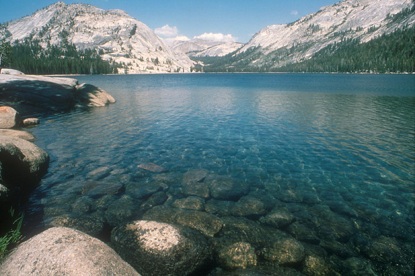
Most people reading this will know that Fresnel reflection is related to the effect on specular objects (i.e most materials we create) where the parts of an object facing us are less reflective, and at grazing angles become more reflective. In fact, at a 90° angle from our eye/camera, all objects reflect 100% of light that hits them and act as a mirror. We can see this clearly in nature when looking at a flat body of water; the water further away from us is more reflective, whilst we can easily look right through the water closest to us. The effect is less noticeable on a rough ocean, where the viewing angle at each point is different – this is also why the Fresnel effect is less noticeable on rough objects. [5]

TenayaLakeTenaya Lake, Yosemite National Park

We can see the fact that 100% of light is reflected at 90° using measured data from refractiveindex.info – a database of different measured materials and their reflectance at different angles and wavelengths. Here is the reflectance of water from 0° to 90°, where the reflectance goes from about 2% to 100% (ignore S-polarised and P-polarised light, here we only care about non-polarised):

reflectance (1)

To prove that this is true for all objects, here is a completely different material, aluminium (note the very different response curve, metals react very differently but are still 100% reflective at a grazing angle):

reflectance

So, why does this happen? When light moves from one medium to another, the light changes speed. Because light will always travel the shortest possible path, this change in speed causes the light to change direction. We describe the ratio of the speed of light from one medium to another as the index of refraction or IOR, mathematically noted as η (“eta”). In CG we almost always treat the first medium, the “air” as a vacuum. So in CG when we talk about IOR we are talking about the ratio of the speed of light in a vacuum to the speed of light inside the medium the light ray is entering. When this occurs, some of the light may be transmitted (refracted) into the medium; the smaller the angle of incidence (the angle between the viewer and the surface normal), the more light that gets transmitted. Due to the law of Conservation of Energy (the total amount of energy must remain constant), the rest of the light will be reflected, as the sum of transmitted and reflected light must be equal to the amount of incident light. [6]

fresnelDiagram.png

This proportion of reflected vs. transmitted light is given by the Fresnel intensity equations, and the amount of reflected light given by these equations is our Fresnel reflection. The Fresnel intensity equations take the angle of the incident ray to the normal of the surface and the refractive indices of both mediums as parameters and output the amount of light to be reflected and the amount of light to be refracted. From these parameters we can also calculate the angles of both reflection and refraction, however the angle of reflection is only dependent on the normal and angle of incidence, whereas refraction depends on the indices of refraction on top of this. Changing your IOR does NOT effect angle of reflection, but does effect angle of refraction. The angle of refraction is given by Snell’s Law which I won’t cover here, but I’ve included reference at the bottom – the only purpose of the Fresnel intensity equations is calculating the ratio of transmitted vs reflected light. [7]

ior
IOR values for different transmissive media (top to bottom) – ice (1.31), crown glass (1.52), flint glass (1.8), and diamond (2.41)
Note how the reflections change in intensity but not shape, but the refractions do change shape

Some shaders do not use an IOR parameter for Fresnel reflections, and decide to use the possibly more intuitive concept of reflectance at facing-angle (this may come under different names such as “f0”, “reflectance at normal”, etc, but is equivalent in each). This gives the user control over what ratio of light is reflected at 0° from the camera (f0, or facing-angle), but does the exact same thing as adjusting the IOR. Just as adjusting the IOR will give us different reflectance values at the facing-angle, we can reverse this and figure out the IOR from the reflectance at the facing-angle – for example an IOR of 1.5 will give us a reflectance of 4%, and vice-versa. This is nice because it allows us to map with values between 0 and 1 (as we usually do with our textures), and has a more direct correlation to what we actually see in the shader.

So, hopefully this is a complete enough description of the IOR parameter on many shaders. But, why do some of these shaders IOR parameters have RGB inputs? This is because the reflectance also depends on the wavelength. For dielectrics (non-metals), there is very little change due to wavelength, giving us achromatic reflections, so many shaders use a single value for IOR. However, for metals, we can sometimes get quite different responses at different wavelengths, which is what gives metals coloured reflections. Any Fresnel reflection mode using an RGB IOR will have another parameter, the extinction coefficient, and together they give us a metallic Fresnel curve. When using this mode, specular colour should not be tinted, as colour should come only from these two parameters – this is a much more physically accurate representation of metallic Fresnel as any Fresnel mode using just IOR is only capable of accurately simulating a non-metallic Fresnel curve.

This is where it gets complex…

When light enters a medium, not only may it be transmitted or reflected, but some of it may also be absorbed. Electrical conductors (i.e, metals) have very high absorption (or extinction) rates, so if light is transmitted rather than reflected, it is almost immediately absorbed. This is why metals are always opaque, and no subsurface scattering occurs. To account for this, we can add another parameter, the extinction coefficient. In our Fresnel intensity equations we can take our index of refraction and replace it with a complex index of refraction, η – iκ, where κ (“kappa”) is the complex part that accounts for extinction. If you don’t know what complex numbers are don’t worry as it isn’t important for this explanation, just know that complex numbers are a convenient way to encode the refractive index and extinction coefficient with a single value. This is what gives us the noticeably distinct reflectance curve in metals, with the characteristic dip right before it reaches 100% reflectance at 90°. Dielectrics will have an extinction coefficient of zero. [8]

The extinction coefficient parameter may not be familiar, because many shaders are designed to just take an IOR or “reflectance at facing angle” value. By using high values for either of these or turning Fresnel off and tinting the specular colour we can achieve a metallic look which is often satisfactory. However, the response curve will not exactly match that of an actual, measured metal.

gold
Gold without Fresnel reflections + tinted spec and with RGB IOR + Extinction Coefficient – note the shifts in intensity and colour at glancing angles

Another alternative to this is the Reflectivity / Edge Tint model – two RGB parameters, Reflectivity for reflectance at facing-angle, and Edge Tint to describe the change of colour at grazing angles. This is just a remapping of IOR / extinction coefficient to more intuitive parameters, therefore you can use physically correct colour values to get results that match measured data. This might be preferable because rather than having to copy values from a database or guess at less obvious parameters like extinction coefficient, you can paint maps with artistic / guessed values and still have metals that react with that characteristic metallic Fresnel curve. For dielectrics, Edge tint is simply left black, and Reflectivity uses achromatic values.

Screen Shot 2018-03-28 at 21.01.47

As mentioned earlier, metals have different responses at different wavelengths, but how this relates to an RGB colour might not be very clear. Calculating these RGB values requires calculating a spectrum and doing multiple conversions based on a colour profile, which is outside of the scope of this lesson. However, it is possible to roughly approximate Reflectivity and Edge Tint by going to refractiveindex.info, entering 0.65, .55 and .44 µm (micrometre) wavelengths for red, green and blue respectively, and using the values given by the reflection calculator for R (non-polarised) at 0° incidence for Reflectivity, and 80° for Edge Tint. Again, this is just a vague approximation, and accurate results require spectral calculations. [10]

Metallic

Common in real-time PBR engines, the metallic or metalness parameter is used to simplify Fresnel for artists, whilst also allowing for optimisation in real-time rendering. However, this parameter is also seen in offline renderers. As metals tend to have little to no diffuse component and dielectrics have grey reflections, we can use a single colour, often called “base color” for our materials. For metallic surfaces the “base color” is used for reflectivity at facing-angle (in game engines often called specular color), and for dielectrics it is used for diffuse colour. Often for dielectrics there is limited control over the IOR – for example, Substance Designer allows for a small range of adjustment, and Painter uses an IOR of 1.5 for all dielectrics. Often this is fine because the range of IOR for dielectrics is quite limited, from about 1.33 to 2, or 2% reflectivity at facing-angle to 11%, but usually hanging around 1.5 IOR. However to get an accurate representation this makes a big difference so it is worth playing with if you have the option. This model is often paired with the Fresnel Schlick approximation, a cheaper approximation of Fresnel that introduces some error but works well for standard dielectric values. [8] [11] Note that metallic maps should be black and white, with grey values only used for anti-aliasing. For example, grey values are acceptable in areas where the microsurface has both metallic and non-metallic areas within one pixel and we don’t have the required resolution to separate them, as opposed to a material that is somewhere in between the two.

So, there it is – a lot of different set-ups, but I believe understanding how specular Fresnel works and what your parameters are doing it should make it much easier to achieve the look you want without too much guesswork. Thanks to Vincent Dedun for proofreading this for me and helping to remove some embarrassing mistakes 🙂

References and Further Reading

[1] https://support.solidangle.com/display/AFMUG/Specular
[2] https://rmanwiki.pixar.com/display/REN/PxrSurface#PxrSurface-SpecularandRoughSpecularParameters
[3] https://docs.redshift3d.com/display/RSDOCS/Material?product=maya#Material-Reflection
[4] https://academy.allegorithmic.com/courses/b6377358ad36c444f45e2deaa0626e65
[5] https://www.scratchapixel.com/lessons/3d-basic-rendering/introduction-to-shading/reflection-refraction-fresnel
[6] https://en.wikipedia.org/wiki/Refractive_index
[7] https://en.wikipedia.org/wiki/Snell%27s_law
[8] https://seblagarde.wordpress.com/2013/04/29/memo-on-fresnel-equations/
[9] https://groups.google.com/forum/#!topic/alshaders/IZTbaqJMQBo
[10] http://jcgt.org/published/0003/04/03/paper.pdf
[11] https://disney-animation.s3.amazonaws.com/library/s2012_pbs_disney_brdf_notes_v2.pdf

At A Glance: Slope-Space Integrals for Specular Next Event Estimation

Figure 1.

Anyone who has tried to render caustic reflections off of water or metallic objects will be aware that it can take a very long time for the render to converge to a good solution. This is because Monte Carlo light transport algorithms struggle to find light paths involving specular materials. For example when we render a diffuse surface such as the wooden table in Figure 1, our first ray shot from the camera will hit the table, and then a secondary ray will bounce off in a random direction. Because the light being reflected off of the specular plant pots is being reflected in a very small cone of directions, the likelihood of our secondary ray shooting in the correct direction to get a significant contribution from the plant pots is very small. However, the specular light reflecting off of the plant pots onto the table is very bright, and so as we only get a few hits here and there, we end up with noisy caustic reflections. What we need to do is come up with away to shoot in these directions with a higher probability.

In a recent paper, Loubet et al. come up with a way to predict the radiance from a specular triangle, and show how thiscan be used to efficiently sample connections between meshes made of millions of triangles. First, they choose a triangleon a specular object based on its total contribution. Then, they sample a position within the triangle – sampling the mostrelevant area in the triangle is important as the region of the triangle making a significant contribution will usually be muchsmaller than the triangle itself.

To solve both of these steps, they do calculations in the space of “microfacet slopes”, or what they call “slope-space”. The term “microfacet” refers to specular reflection models which approximate reflections off of surfaces as distributions of millions of microscopic mirrors, or microfacets, on the surface. The statistical distribution of the directions of these microfacets determines the appearance of the reflection – some distributions you may have heard of include GGX, Beckmann, and Ward.

Figure 2.

Previous work such as Olano and Baker’s 2010 paper on LEAN Mapping involves blending the contributions of bump maps into the microfacets as the surface moves further away from the camera. As the camera moves away, the bump details are filtered out, so moving those details into the microfacets preserves them. To achieve this, they introduce the concept of “off-center” microfacet models, where the average direction of the microfacets differs from the surface normal. To work with these models, Olano and Baker transform the microfacets into a common space, referred to here as “slope-space”, which allows them to do things such as combining the results of multiple bump maps with the microfacets. Transforming into slope-space involves projecting the directions from the surface onto a plane tangent to it (Figure 2). Loubet et al. build on this work, using slope-space to simplify their own calculations.

So, the first step; predicting the radiance from a specular triangle. Using the example of our wooden table and specular pots shown in Figure 1, we need to find the amount of light that is reflected into our camera from a point on the table, after it has been reflected by a specular triangle belonging to a pot. In the paper, they assume that specular roughness is constant over the triangle, and the triangle has shading normals defined at its vertices. Calculating the amount of radiance requires several key ingredients;
● The set of directions from the triangle to the point on the table
● The set of directions from the light source to the triangle
● The result of the BSDF (shader) at the point on the table
● The accumulated result (integral) of the BSDF over the triangleS

Solving this is very difficult for a couple of reasons. The first is that the directions to and from the triangle vary spatially over the triangle in a “non-linear” way, meaning that it is hard to calculate without just taking lots of samples, which is extremely slow. To work around this, Loubet et al. use “far-field approximation”, where they assume that the triangle is significantly distant from both the light source and the point on the table, and therefore the directions will vary by negligible amounts – similar to how we might use a directional light to simulate the sun. This assumption holds if the triangle is either far away from both points or is relatively small. To ensure this, they subdivide the triangle into smaller triangles until the triangle being looked at can be approximated to an acceptable degree.

This approximation makes everything straightforward to compute, other than the last element on our list; the integral of the BSDF over the triangle. The BSDF over the triangle is still spatially varying, because the 3 shading normals defined at the vertices of the triangle are interpolated over the triangles surface. This means that the average direction of the microfacets over the triangle can change a lot, which is something we don’t want to neglect, as getting an accurate specular response is essential.

Figure 3.
Figure 4.

When we compare the shading normals, we can see that they define a spherical triangle of directions (the blue triangle in Figure 3) over which we need to integrate the BSDF. There is no way to calculate this directly, so we need a clever solution. In the paper they give the specular triangle an off-center microfacet BSDF, which allows them to define the shading normals in slope-space. To transform into slope-space, the 3D normals are projected onto a plane, becoming 2D points (Figure 3). Therefore our spherical triangle is projected as a 2D shape in slope-space. They show that it is possible to directly calculate the result in slope-space as long as the shading normals vary linearly within the projection. Although they do not actually vary linearly in slope-space, they show that as long as the triangle is sufficiently small / distant, linear interpolation in slope-space (the red triangle in Figure 3) is a very close approximation. In Figure 4, we see that linear interpolation matches well on a distant projected spherical triangle (left), but not well on a close one (right). This works in our case, because we are already assuming small / distant triangles.

Ta-dah! We now have a way to efficiently approximate the total amount of radiance reflected by a triangle from one point to another, as well as an approximate distribution over the whole triangle. As this is after all just an approximation, instead of using this result directly we can use it to take more samples in the area of the triangle with the biggest approximated impact (this is known as “importance sampling”). Loubet et al. use this result to create a new “Next Event Estimation” (NEE) strategy, which they call “Specular Next Event Estimation” (SNEE). NEE involves reusing found light paths, by drawing connections from every ray hit from indirect bounces to the light sources. This means we get more bang for our buck for each ray we shoot, speeding up render times significantly. In contrast, SNEE involves finding sub-paths between the specular triangles in the scene and the light sources, rather than direct connections.

If we were to do this naively, we would shoot a ray at a point to be shaded from our camera, randomly select a point on a light source, estimate the contribution of all specular triangles in the scene reflecting light from the light source onto the point being shaded, and finally importance sample one of the triangles that makes some significant contribution. In a standard scene with millions of triangles, this will be very slow. To address this they build a hierarchical data structure in a pre-rendering step, where they trace rays from the light sources to each specular triangle at random points. For each triangle, they calculate reflection and refraction bounces and store all intersections with non-specular geometry in two bounding boxes with the associated amount of energy; one for reflections, and another for refractions. All of these bounding boxes are then stored in a weighted bounding volume hierarchy (BVH), which can then be used to efficiently search for specular paths.

Figure 5.
Figure 6.

The results are really impressive; they rendered the plant pot scene in 30 minutes, and the turtle scene (Figure 5) in just 5 minutes! They also use similar techniques to efficiently render high frequency normal maps on specular surfaces (Figure 6). The algorithm is unbiased, and works with standard unidirectional path-tracing. The biggest limitation with SNEE is that it only works on specular paths with a single bounce, so adding more bounces will be the next big step for improving this method.

That about wraps it up for this one, I really hope you found it interesting. Perhaps we will see these techniques coming to a path-tracer near you within the next few years!

At A Glance: Neural Scene Representations + An Interview with Jonathan Granskog (NVIDIA)

A neural network is a representation of individual “neurons” which are connected to each other, inspired by the way our brains work. An input – for example, an image of a dog – is put into the network, leading to a chain of neurons firing off through the network into an output. If we give the neural network a lot of labelled training data, for example thousands of images of cats and dogs labelled “cat” and “dog”, over time it can “learn” the difference between the two, and the output we get from the network will be the word “dog”. This is just a simple example, and the concept can be applied to many, many different applications.

In computer graphics, there has been a great deal of recent research using neural networks to create realistic images. For example, the rendering of completely believable human faces and relighting of existing images. There has also been amazing work done on light transport. Neural networks are used regularly in production today to denoise renders (the OptiX AI denoiser for example), using AOVs containing information about the scene to clean up the final image. Taking this a step further, recent research has used a “neural renderer” to infer the shading for the image based on just the AOVs alone. The issue with using a screen-space neural renderer such as this however, is that it is unable to account for effects caused by objects outside of the camera’s view. As well as this, the neural network performs all of this work at once. The neural network becomes a “black box”; it is hard to interpret exactly what it is doing and how it is doing it, and difficult to understand where it’s weaknesses are and how it can be improved.

To improve on this, when using a neural renderer we can break the task into first creating a neural representation of the scene, and then use that scene representation to render an image. A separate neural network is given a few renders and G-buffers from different viewpoints of the scene, and creates an abstract representation of that scene. All the neural renderer then requires is the scene representation, a camera transform, and geometric AOVs (normals, positions, etc. – known collectively as the “G-buffer”) for that viewpoint. We can now account for objects outside of our field of view, and we also have more control over how we render the image. For example, we could impose physically-based constraints, and ensure consistency between different views of the scene. The neural scene could also be used to complement our traditional rendering pipelines, for example we could use a raytracer to quickly calculate direct lighting, and use the neural renderer to quickly infer global illumination. Using a neural scene representation, we have gained more control over how our scene is rendered, however the scene itself is still somewhat of a black box. If we see any incorrect artifacts in our image, it is not obvious what we must change in our neural scene representation to account for them.

A recent paper in this area was presented at this year’s SIGGRAPH conference. This paper is a step towards having finer-grained control over this neural scene representation, where the geometry, materials and lighting of the scene are separated from each other. Using this scene representation, it is much easier to troubleshoot where rendering artifacts and poor performance are coming from. During research, for example, they were able to look at problematic regions of their rendered images, noticed a lack of geometric information, and were able to address the issues. Another advantage gained from partitioning the scene representation like this is that the scene can be compressed, by adding a fourth, empty partition which is encouraged to grow to a certain size during training, shrinking the other 3. The bigger the empty partition, the smaller the scene, although the less accurate the output. Different scenes can also be composited with each other in different ways; an example is given of using the lighting of one scene and applying it to another.

Jonathan Granskog is a research scientist at Nvidia, who is the lead author of this paper. He has very kindly allowed me to ask him a few questions about it!

What do you see as being the next step for finer-grained control over these neural scene representations?

In our paper, we focused on splitting the representation into material, lighting and geometry partitions. This enables some user control, but it’s still lacking in terms of the control artists want. As a next step, I would like to see intuitive control of transforms and material parameters of individual objects in the scene.

In the examples, you show not only the lighting of a scene being applied to another, but even interpolating between the lighting of different scenes and applying it to another scene. Is it possible to apply geometry or materials from one scene to another in this way?

Material transfer is definitely possible and something we tried, but decided not to include in the paper because relighting felt more useful and intuitive. Geometry interpolation unfortunately does not work correctly when we give the G-buffer as input. You could update the G-buffer as you interpolate, however there is nothing that enforces that a linearly interpolated representation results in linearly interpolated geometry. You could train a generator without any G-buffer input at all but this is very slow currently (see Neural Scene Representation and Rendering from Eslami et al.).

Are you able to interactively produce final images? Is it close to real-time?

I don’t remember specific timings, but I think we got around 10fps at 256×256 which is not real-time yet but interactive. This is still using research code and you would get a lot faster inference times with more optimisation. We still have a long way to go though until it’s real-time at 1080p.

Do you see any of these techniques potentially being used in VFX/animation workflows in the near or distant future? Which fields do you think they could potentially have the biggest impact upon?

My hope is that in around 5 years time these methods will find their way into 3D applications as a way of quickly approximating slow global illumination. But another application would be specialised neural renderers for example for architectural visualisation. The network learns what typical ArchViz scenes look like and can therefore render high-quality images of these interactively. Now, this would have a big impact considering how many people create these types of images day to day. This idea was actually the inspiration for the ArchViz scene we created for the paper.

But in general, neural scene representations could already be useful in VFX. We already have neural denoisers running in many 3D applications that always use screen-space information meaning the network won’t know about the things not visible to the camera. This could potentially lead us to failing to reconstruct an important caustic effect.

What were your favourite papers from this year’s SIGGRAPH?

Hmmm… I haven’t read many of this year’s SIGGRAPH papers yet. It’s still on my TO DO list. 🙂 All of the presentations I watched during the conference were very high-quality and there was a lot of good research this year. Some of my favorite presentations were:

Consistent Video Depth Estimation
Neural Supersampling for Real-time Rendering
Radiative Backpropagation: An Adjoint Method for Lightning-Fast Differentiable Rendering
Spatiotemporal Reservoir Resampling for Real-Time Ray Tracing With Dynamic Direct Lighting
Specular Manifold Sampling for Rendering High-Frequency Caustics and Glints
Learning Temporal Coherence via Self-Supervision for GAN-Based Video Generation

In particular, I was a big fan of all the differentiable rendering content this year and I believe the technology will be greatly impactful in many fields. There was a 3-hour course that I enjoyed a lot: https://shuangz.com/courses/pbdr-course-sg20/

Poor Man’s Photogrammetry Rig

I recently put together a cheap set-up for photogrammetry, and I’m surprised by the quality of results I was able to get with such a simple set-up. It consists of 5 cheap blank canvases stuck together to build the walls and diffuse light, 2 cheap LED lights, a fidget spinner and CD-ROM to form the base, and a receipt spike for propping up the object being scanned. Still needs some work but pretty happy with how quickly I was able to get to this point.

Shot on a Canon 500D, created using Agisoft Photoscan, Photoshop and ZBrush (the not-so-cheap parts).

IMG_6107lookdevlookdev_grey

At A Glance: Monte Carlo Geometry Processing

This year a paper was published that a lot of people seemed to be going crazy over – the day it was published, I saw several implementations on Twitter, and lots of comments getting excited over the possible applications. So I took a look, and found I had no idea what anyone was talking about! Hardly that surprising as I’m a lookdev artist, not a researcher/developer. But writing these little articles has been a great excuse to go a little deeper into things I am curious about, so here’s my attempt to dive in and understand what all of the fuss is about!

Geometry processing is an area of research concerned with efficient algorithms which are used in ray-tracing, photogrammetry, fluid simulations, path-finding, deformation and more. Many of these tasks involve solving complicated equations that deal with relationships between different functions with multiple variables – known as Partial Differential Equations (PDEs) – which are generally very hard to solve. Therefore we traditionally simplify the geometry into smaller, simpler parts – usually triangles – where we can solve the PDEs more easily. This process is known as “meshing”. We might generate our new triangle mesh from a much higher resolution one, CAD data, a point cloud, or implicit surfaces (surfaces which are defined by equations, as opposed to data). This process of taking a larger problem and breaking it into more manageable pieces is known as a Finite Element Method (FEM).

Meshing, however, has a lot of issues. Creating a high quality mesh can be difficult, and bad meshes can create issues down the line. Even the most robust methods often lose important geometric detail, and depending on the quality of the input may be slow. In fact meshing is usually the main bottle-neck – actually solving the PDEs generally does not take long once the meshing is completed. The traditional methods have other issues too; they introduce error as they only approximate the geometry, and involve solving a large system of equations for the whole of the geometry, even if we are only interested in a small section of it.

This paper attempts to solve these issues and more by introducing the concept of Monte Carlo geometry processing. Monte Carlo integration involves taking a number of random samples and averaging them out to approximate the solution to an equation – usually where the equation is difficult or even impossible to solve by standard integration. With enough random samples the output will eventually converge to the correct result, although too few samples will result in a lot of variation around the true function, or “noise”. Monte Carlo methods are used extensively in rendering today to calculate the global illumination in a scene, where it’s necessary but difficult to calculate the light hitting and reflecting off of surfaces from a huge number of directions. In the paper, they apply these methods to approximate the geometry where needed, rather than breaking the entire thing down into triangles. Interestingly, in the past the more popular method of calculating global illumination was using FEMs, but today FEMs have been overtaken by Monte Carlo integration because of its relative simplicity, accuracy, and efficiency with modern computers – so going in a similar direction for geometry processing seems like it could also have a big impact.

An example is given where they use these methods to solve the “Laplacian” of a point inside some given geometry. The Laplacian is a PDE whose solution can be used to interpolate some surface function into the interior, for example the surface colour. This PDE is used very commonly in geometry processing. To solve it using Monte Carlo methods we can take a large number of “random walks” – this is where small steps are taken from a point inside of the geometry in random directions until we reach the surface – and take the average the colours that we get at the surface, which will give us the interpolated colour at that point. Unfortunately, simulating all of those random steps would be extremely expensive to compute.

An interesting property of this function is that the colour at a given point inside of the geometry is equal to the average colour on the surface of any sphere centred around that point. Therefore, if we perform random walks from our point onto that sphere instead of the geometry itself, our colour will still average out to the solution at that point. In the paper, they start with a sphere around the point to be solved, making it as large as possible to still fit within the geometry. To find the colour of the points on that sphere, we can perform random walks onto other spheres centred at those points, and so on. As we go on, the spheres get smaller and smaller, and their centres get closer to the surface. When we get close enough to some point on the surface of the geometry, we can sample the colour. The likelihood of a random walk exiting at any point of the sphere is the same as any other, as the sphere is perfectly symmetrical – so instead of doing a random walk, we can simply choose a random point on the sphere, which will statistically give us the same result, and be much faster. This method is called “walk on spheres”, and by using it they can solve the Laplacian on many different types of geometry, without the need for meshing! This technique can be generalised, and used to solve many other PDEs as well.

Using this method, booleans can easily be performed between different types of geometry, and the results are efficient and accurate regardless of the quality of the input geometry (imagine using booleans between two pieces of low quality geometry in Maya – you won’t get a great result). The method is also highly parallelisable – meshing generally needs to be done all at once, whereas random samples used for Monte Carlo methods can be taken at the same time – similar to how path tracing is well suited to high thread count CPUs and GPUs, this method is as well.

Many of the advantages of Monte Carlo methods used in rendering can also be applied here – adaptive sampling (taking more samples in areas where there is more noise, seen in V-Ray for example), no ceiling for quality of the approximation (the quality of the approximation depends only on the number of samples taken, and will always converge to the correct result), and denoising can be used as well! There have already been a lot of interesting uses so I recommend Googling if you are interested!

Special Delivery

Since finishing uni I’ve been working at Aardman Animations as a Technical Co-Ordinator on this 360 degree interactive Christmas short for Google! I’m posting this somewhat late after Christmas but have decided to start posting here more after uni. Please give it a watch and let me know what you think!

NOTE: This will run correctly only on supported devices (multiple phones and tablets). If you’re not on a supported device, it will redirect you to a pre-recorded 360 degree YouTube video, but you’ll still get an idea of what it’s like 🙂